7  Building Reproducible Pipelines with rixpress

7.1 Introduction: From Scripts and Notebooks to Pipelines

With reproducible environments (Nix, {rix}), functional code (Chapter 5), and testing skills (Chapter 6) in hand, we’re now ready to orchestrate complete analytical pipelines. But there’s one more piece to the puzzle: orchestration.

How do we take our collection of functions and data files and run them in the correct order to produce our final data product? This problem of managing computational workflows is not new, and a whole category of build automation tools has been created to solve it.

7.1.1 The Evolution of Build Automation

The original solution, dating back to the 1970s, is make. Created by Stuart Feldman at Bell Labs in 1976, make reads a Makefile that describes the dependency graph of a project. If you change the code that generates plot.png, make is smart enough to only re-run the steps needed to rebuild the plot and the final report.

The strength of these tools is their language-agnosticism, but their weaknesses are twofold:

1. File-centric: You must manually handle all I/O. Your first script saves data.csv, your second loads it. This adds boilerplate and creates surfaces for error.
2. Environment-agnostic: They track files but know nothing about the software environment needed to create those files.

This is where R’s {targets} package shines. It tracks dependencies between R objects directly, automatically handling serialisation. But {targets} operates within a single R session; for polyglot pipelines, you must manually coordinate via {reticulate}.

7.1.2 The Separation Problem

All these tools (from make to {targets} to Airflow) separate workflow management from environment management. You use one tool to run the pipeline and another (Docker, {renv}) to set up the software.

This separation creates friction. Running {targets} inside Docker ensures reproducibility, but forces the entire pipeline into one monolithic environment. What if your Python step requires TensorFlow 2.15 but your R step needs reticulate with Python 3.9? You’re stuck.

7.1.3 The Imperative Approach: Make + Docker

To illustrate this, consider the traditional setup for a polyglot pipeline. You’d need:

1. A Dockerfile to set up the environment
2. A Makefile to orchestrate the workflow
3. Wrapper scripts for each step

Here’s what a Makefile might look like:

# Makefile for a Python → R pipeline

DATA_DIR = data
OUTPUT_DIR = output

$(OUTPUT_DIR)/predictions.csv: $(DATA_DIR)/raw.csv scripts/train_model.py
python scripts/train_model.py $(DATA_DIR)/raw.csv $@

$(OUTPUT_DIR)/plot.png: $(OUTPUT_DIR)/predictions.csv scripts/visualise.R
Rscript scripts/visualise.R $< $@

$(OUTPUT_DIR)/report.html: $(OUTPUT_DIR)/plot.png report.qmd
quarto render report.qmd -o $@

all: $(OUTPUT_DIR)/report.html

clean:
rm -rf $(OUTPUT_DIR)/*

This looks clean, but notice the procedural boilerplate required in each script. Your train_model.py must parse command-line arguments and handle file I/O:

# scripts/train_model.py
import sys
import pandas as pd
from sklearn.ensemble import RandomForestClassifier

def main():
    input_path = sys.argv[1]
    output_path = sys.argv[2]

    # Load data
    df = pd.read_csv(input_path)

    # ... actual ML logic ...

    # Save results
    predictions.to_csv(output_path, index=False)

if __name__ == "__main__":
    main()

And your visualise.R script needs the same boilerplate:

# scripts/visualise.R
args <- commandArgs(trailingOnly = TRUE)
input_path <- args[1]
output_path <- args[2]

# Load data
predictions <- read.csv(input_path)

# ... actual visualisation logic ...

# Save plot
ggsave(output_path, plot)

The scientific logic is buried under file I/O scaffolding. And the environment? That’s a separate 100+ line Dockerfile you must maintain.

7.1.4 rixpress: Unified Orchestration

This brings us to a key insight: a reproducible pipeline should be nothing more than a composition of pure functions, each with explicit inputs and outputs, no hidden state, and no reliance on execution order beyond what the data dependencies require.

{rixpress} solves this by using Nix not just as a package manager, but as the build automation engine itself. Each pipeline step is a Nix derivation: a hermetically sealed build unit.

Compare the same pipeline in {rixpress}:

library(rixpress)

list(
  rxp_py_file(
    name = raw_data,
    path = "data/raw.csv",
    read_function = "lambda x: pandas.read_csv(x)"
  ),

  rxp_py(
    name = predictions,
    expr = "train_model(raw_data)",
    user_functions = "functions.py"
  ),

  rxp_py2r(
    # rxp_py2r uses reticulate for conversion
    name = predictions_r,
    expr = predictions
  ),

  rxp_r(
    name = plot,
    expr = visualise(predictions_r),
    user_functions = "functions.R"
  ),

  rxp_qmd(
    name = report,
    qmd_file = "report.qmd"
  )
) |>
  rxp_populate()

And your functions.py contains only the scientific logic:

# functions.py
def train_model(df):
    # ... pure ML logic, no file I/O ...
    return predictions

The difference is stark:

Aspect	Make + Docker	rixpress
Files needed	Dockerfile, Makefile, wrapper scripts	gen-env.R, gen-pipeline.R, function files
I/O handling	Manual in every script	Automatic via encoders/decoders
Dependencies	Explicit file rules	Inferred from object references
Environment	Separate Docker setup	Unified via {rix}
Expertise needed	Linux admin, Make syntax	R programming

This provides two key benefits:

1. True Polyglot Pipelines: Each step can have its own Nix environment. A Python step runs in a pure Python environment, an R step in an R environment, a Quarto step in yet another, all within the same pipeline. Julia is also supported, and {reticulate} can be used for data transfer, but arbitrary encoder and decoder as well (more on this later).

2. Deep Reproducibility: Each step is cached based on the cryptographic hash of all its inputs: the code, the data, and the environment. Any change in dependencies triggers a rebuild. This is reproducibility at the build level, not just the environment level.

The interface is heavily inspired by {targets}, so you get the ergonomic, object-passing feel you’re used to, combined with the bit-for-bit reproducibility of the Nix build system.

TipGetting LLM assistance with {rixpress} and ryxpress

If the {rixpress} syntax is new to you, remember that you can use pkgctx to generate LLM-ready context (as mentioned in the introduction). Both the {rixpress} (R) and ryxpress (Python) repositories include .pkgctx.yaml files you can feed to your LLM to help it understand the package’s API. You can also generate your own context files:

# For the R package
nix run github:b-rodrigues/pkgctx -- r github:b-rodrigues/rixpress > rixpress.pkgctx.yaml

# For the Python package
nix run github:b-rodrigues/pkgctx -- python ryxpress > ryxpress.pkgctx.yaml

With this context, your LLM can help you write correct pipeline definitions, even if the syntax is completely new to you. You can do so for any package hosted on CRAN, GitHub, or local .tar.gz files.

7.2 What is rixpress?

{rixpress} streamlines creation of micropipelines (small-to-medium, single-machine analytic pipelines) by expressing a pipeline in idiomatic R while delegating build orchestration to the Nix build system.

Key features:

• Define pipeline derivations with concise rxp_*() helper functions
• Seamlessly mix R, Python, Julia, and Quarto steps
• Reuse hermetic environments defined via {rix} and a default.nix
• Visualise and inspect the DAG; selectively read, load, or copy outputs
• Automatic caching: only rebuild what changed

{rixpress} provides several functions to define pipeline steps:

Function	Purpose
rxp_r()	Run R code
rxp_r_file()	Read a file using R
rxp_py()	Run Python code
rxp_py_file()	Read a file using Python
rxp_qmd()	Render a Quarto document
rxp_py2r()	Convert Python object to R using reticulate
rxp_r2py()	Convert R object to Python using reticulate

Here is what a basic pipeline looks like:

library(rixpress)

list(
  rxp_r_file(
    mtcars,
    'mtcars.csv',
    \(x) read.csv(file = x, sep = "|")
  ),

  rxp_r(
    mtcars_am,
    filter(mtcars, am == 1)
  ),

  rxp_r(
    mtcars_head,
    head(mtcars_am)
  ),

  rxp_qmd(
    page,
    "page.qmd"
  )
) |>
  rxp_populate()

7.3 Getting Started

7.3.1 Initialising a project

If you’re starting fresh, you can bootstrap a project using a temporary shell:

nix-shell -p R rPackages.rix rPackages.rixpress

Once inside, start R and run:

rixpress::rxp_init()

This creates two essential files:

• gen-env.R: Where you define your environment with {rix}
• gen-pipeline.R: Where you define your pipeline with {rixpress}

7.3.2 Defining the environment

Open gen-env.R and define the tools your pipeline needs:

library(rix)

rix(
  date = "2025-10-14",
  r_pkgs = c("dplyr", "ggplot2", "quarto", "rixpress"),
  ide = "none",
  project_path = ".",
  overwrite = TRUE
)

Run this script to generate default.nix, then build and enter your environment:

nix-build
nix-shell

7.3.3 Defining the pipeline

Open gen-pipeline.R and define your pipeline:

library(rixpress)

list(
  rxp_r_file(
    name = mtcars,
    path = "data/mtcars.csv",
    read_function = \(x) read.csv(x, sep = "|")
  ),

  rxp_r(
    name = mtcars_am,
    expr = dplyr::filter(mtcars, am == 1)
  ),

  rxp_r(
    name = mtcars_head,
    expr = head(mtcars_am)
  )
) |>
  rxp_populate()

Running rxp_populate() generates a pipeline.nix file and builds the entire pipeline. It also creates a _rixpress folder with required files for the project.

You don’t need to write gen-pipeline.R completely in one go. Instead, start with a single derivation, usually the one loading the data, and build the pipeline using source("gen-pipeline.R") and then rxp_make(). Alternatively, if you set build = TRUE in rxp_populate(), sourcing the script alone would be enough, as the pipeline would be built automatically.

In an interactive session, you can use rxp_read(), rxp_load() to read or load artifacts into the R session respectively and rxp_trace() to check the lineage of an artifact. This way, you can also work interactively with {rixpress}: add derivations one by one and incrementally build the pipeline. If you change previous derivations or functions that affect them, you don’t need to worry about re-running past steps—these will be executed automatically since they’ve changed!

7.4 Real-World Examples

The rixpress_demos repository contains many complete examples. Here are a few practical patterns to get you started.

7.4.1 Example 1: Reading Many Input Files

When you have multiple CSV files in a directory:

library(rixpress)

list(
  # R approach: read all files at once
  rxp_r_file(
    name = mtcars_r,
    path = "data",
    read_function = \(x) {
      readr::read_delim(list.files(x, full.names = TRUE), delim = "|")
    }
  ),

  # Python approach: custom function
  rxp_py_file(
    name = mtcars_py,
    path = "data",
    read_function = "read_many_csvs",
    user_functions = "functions.py"
  ),

  rxp_py(
    name = head_mtcars,
    expr = "mtcars_py.head()"
  )
) |>
  rxp_populate()

The key insight: rxp_r_file() and rxp_py_file() can point to a directory, and your read_function handles the logic.

7.4.2 Example 2: Machine Learning with XGBoost

This pipeline trains an XGBoost classifier in Python, then passes predictions to R for evaluation with {yardstick}:

library(rixpress)

list(
  # Load data as NumPy array
  rxp_py_file(
    name = dataset_np,
    path = "data/pima-indians-diabetes.csv",
    read_function = "lambda x: loadtxt(x, delimiter=',')"
  ),

  # Split features and target
  rxp_py(name = X, expr = "dataset_np[:,0:8]"),
  rxp_py(name = Y, expr = "dataset_np[:,8]"),

  # Train/test split
  rxp_py(
    name = splits,
    expr = "train_test_split(X, Y, test_size=0.33, random_state=7)"
  ),

  # Extract splits

  rxp_py(name = X_train, expr = "splits[0]"),
  rxp_py(name = X_test, expr = "splits[1]"),
  rxp_py(name = y_train, expr = "splits[2]"),
  rxp_py(name = y_test, expr = "splits[3]"),

  # Train XGBoost model
  rxp_py(
    name = model,
    expr = "XGBClassifier(use_label_encoder=False, eval_metric='logloss').fit(X_train, y_train)"
  ),

  # Make predictions
  rxp_py(name = y_pred, expr = "model.predict(X_test)"),

  # Export predictions to CSV for R
  rxp_py(
    name = combined_df,
    expr = "DataFrame({'truth': y_test, 'estimate': y_pred})"
  ),

  rxp_py(
    name = combined_csv,
    expr = "combined_df",
    user_functions = "functions.py",
    encoder = "write_to_csv"
  ),

  # Compute confusion matrix in R
  rxp_r(
    combined_factor,
    expr = mutate(combined_csv, across(everything(), factor)),
    decoder = "read.csv"
  ),

  rxp_r(
    name = confusion_matrix,
    expr = yardstick::conf_mat(combined_factor, truth, estimate)
  )
) |>
  rxp_populate(build = FALSE)

# Adjust Python imports
adjust_import("import numpy", "from numpy import array, loadtxt")
adjust_import("import xgboost", "from xgboost import XGBClassifier")
adjust_import("import sklearn", "from sklearn.model_selection import train_test_split")
add_import("from pandas import DataFrame", "default.nix")

rxp_make()

This demonstrates:

• Python-heavy computation with XGBoost
• Custom serialization via encoder/decoder
• Adjusting Python imports with adjust_import() and add_import()
• Passing results to R for evaluation

7.4.3 Example 3: Simple Python→R→Quarto Workflow

A complete pipeline that bounces data between languages and renders a report:

library(rixpress)

list(
  # Read with Python polars
  rxp_py_file(
    name = mtcars_pl,
    path = "data/mtcars.csv",
    read_function = "lambda x: polars.read_csv(x, separator='|')"
  ),

  # Filter in Python, convert to pandas for reticulate
  rxp_py(
    name = mtcars_pl_am,
    expr = "mtcars_pl.filter(polars.col('am') == 1).to_pandas()"
  ),

  # Convert to R
  rxp_py2r(name = mtcars_am, expr = mtcars_pl_am),

  # Process in R
  rxp_r(
    name = mtcars_head,
    expr = my_head(mtcars_am),
    user_functions = "functions.R"
  ),

  # Back to Python
  rxp_r2py(name = mtcars_head_py, expr = mtcars_head),

  # More Python processing
  rxp_py(name = mtcars_tail_py, expr = "mtcars_head_py.tail()"),

  # Back to R
  rxp_py2r(name = mtcars_tail, expr = mtcars_tail_py),

  # Final R step
  rxp_r(name = mtcars_mpg, expr = dplyr::select(mtcars_tail, mpg)),

  # Render Quarto document
  rxp_qmd(
    name = page,
    qmd_file = "my_doc/page.qmd",
    additional_files = c("my_doc/content.qmd", "my_doc/images")
  )
) |>
  rxp_populate()

Note the additional_files argument for rxp_qmd(): this includes child documents and images that the main Quarto file needs.

7.5 Working with Pipelines

7.5.1 Building the pipeline

You can build the pipeline in two steps:

# Generate pipeline.nix only (don't build)
rxp_populate(build = FALSE)

# Build the pipeline
rxp_make()

Or in a single step with rxp_populate(build = TRUE). Once you’ve built the pipeline, you can inspect the results.

7.5.2 Inspecting outputs

Because outputs live in /nix/store/, {rixpress} provides helpers:

# List all built artifacts
rxp_inspect()

# Read an artifact into R
rxp_read("mtcars_head")

# Load an artifact into the global environment
rxp_load("mtcars_head")

It is important to understand that all artifacts are stored in the /nix/store/. So if you want to save the outputs somewhere else, you need to use rxp_copy().

rxp_copy("clean_data")

This will copy the clean_data artifacts into the current working directory. If you call rxp_copy() without arguments, every artifact will be copied over.

Over time, the Nix store can accumulate many artifacts from previous pipeline runs. Use rxp_gc() to clean up old build outputs and reclaim disk space:

# Preview what would be deleted (dry run)
rxp_gc(keep_since = "2026-01-01", dry_run = TRUE)

# Delete artifacts older than a specific date
rxp_gc(keep_since = "2026-01-01")

# Full garbage collection (removes all unreferenced store paths)
rxp_gc()

The keep_since argument lets you preserve recent builds while cleaning up older ones. This is particularly useful on shared machines or CI runners where disk space is limited.

7.5.3 Visualising the pipeline

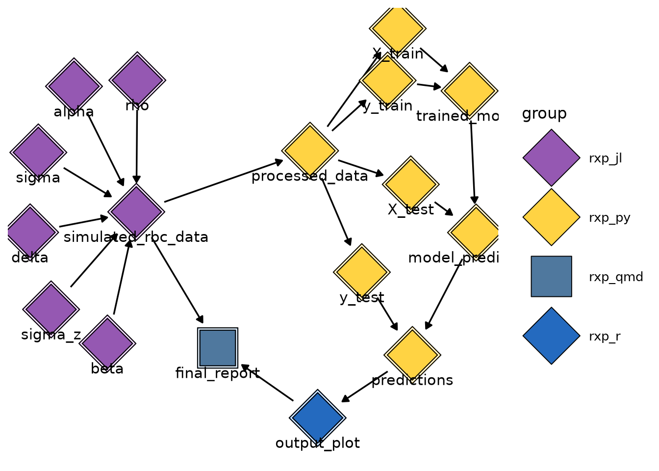
There are three ways to visualise pipelines. The first is to look at the trace of a derivation or of the full pipeline. This is similar to a genealogy tree. You can start by running rxp_inspect() to double check how the derivation names are written:

rxp_inspect()

derivation build_success
1              X_test          TRUE
2             X_train          TRUE
3               alpha          TRUE
4                beta          TRUE
5     all-derivations          TRUE
6               delta          TRUE
7        final_report          TRUE
8   model_predictions          TRUE
9         output_plot          TRUE
10        predictions          TRUE
11     processed_data          TRUE
12                rho          TRUE
13              sigma          TRUE
14            sigma_z          TRUE
15 simulated_rbc_data          TRUE
16      trained_model          TRUE
17             y_test          TRUE
18            y_train          TRUE

Let’s check the trace of output_plot:

rxp_trace("output_plot")

==== Lineage for: output_plot ====
Dependencies (ancestors):
  - predictions
    - y_test*
      - processed_data*
        - simulated_rbc_data*
          - alpha*
          - beta*
          - delta*
          - rho*
          - sigma*
          - sigma_z*
    - model_predictions*
      - X_test*
        - processed_data*
      - trained_model*
        - X_train*
          - processed_data*
        - y_train*
          - processed_data*

Reverse dependencies (children):
  - final_report

Note: '*' marks transitive dependencies (depth >= 2).

We see that output_plot depends directly on predictions, and predictions on y_test, which itself depends on all the other listed dependencies. The children of the derivation are also listed, in this case final_report.

Calling rxp_trace() without arguments shows the entire pipeline:

rxp_trace()

- final_report
  - simulated_rbc_data
    - alpha*
    - beta*
    - delta*
    - rho*
    - sigma*
    - sigma_z*
  - output_plot
    - predictions*
      - y_test*
        - processed_data*
          - simulated_rbc_data*
      - model_predictions*
        - X_test*
          - processed_data*
        - trained_model*
          - X_train*
            - processed_data*
          - y_train*
            - processed_data*

Note: '*' marks transitive dependencies (depth >= 2).

Another way to visualise the pipeline is by using rxp_ggdag(). This requires the {ggdag} package to be installed in the environment. Calling rxp_ggdag() shows the following plot:

Derivations are coloured by programming language.

Finally, you can also use rxp_visnetwork() (which requires the {visNetwork} package). This opens an interactive JavaScript visualization in your browser, allowing you to zoom into and explore different parts of your pipeline.

7.5.4 Caching, Incremental Builds and Build Logs

One of the most powerful features of using Nix for pipelines is automatic caching. Because Nix tracks all inputs to each derivation, it knows exactly what needs to be rebuilt when something changes.

Try this:

1. Build your pipeline with rxp_make()
2. Change one step in your pipeline
3. Run rxp_make() again

Nix will detect that unchanged steps are already cached and instantly reuse them. It only rebuilds the steps affected by your change. Also, your pipeline is actually also a child of the environment. So if the environment changes (for example, you update the date argument in the rix() call), your entire pipeline will be rebuilt. While this might seem like overkill, this is actually the only way you can guarantee that the pipeline is reproducible and works. If the pipeline weren’t rebuilt when updating the environment, and cached results were re-used, you’d never know if a non-backwards-compatible change in a function in some package would break your pipeline!

Every time you run rxp_populate(), a timestamped log is saved in the _rixpress/ directory. This is like having a Git history for your pipeline’s outputs. Suppose I update a derivation in my pipeline, and build the pipeline again. Calling rxp_list_logs() shows me this:

rxp_list_logs()

> rxp_list_logs()
filename
1 build_log_20260131_104726_bpjnnq2nax40w45rzbl83ggp5y766dsv.json
2 build_log_20260131_101941_y4gz22nl1aym5yfzp3wgj5glmzv3wx5v.json
modification_time size_kb
1 2026-01-31 10:47:26    3.06
2 2026-01-31 10:19:41    3.06

I also recommend committing the change, so the time of the rixpress log matches the time of the change:

git log

commit 043dd99cb56966af449796f636470462b5624d85
Author: Bruno Rodrigues <bruno@brodrigues.co>
Date:   Sat Jan 31 10:46:02 2026 +0100

  updated alpha from 0.3 to 0.4

I can now update the derivation again, and rebuild the pipeline. rxp_list_logs() shows the following:

                                                         filename
1 build_log_20260131_110120_v470crwiqx2k0g5bfvd4mqm73ssjdaa5.json
2 build_log_20260131_104726_bpjnnq2nax40w45rzbl83ggp5y766dsv.json
3 build_log_20260131_101941_y4gz22nl1aym5yfzp3wgj5glmzv3wx5v.json
    modification_time size_kb
1 2026-01-31 11:01:20    3.06
2 2026-01-31 10:47:26    3.06
3 2026-01-31 10:19:41    3.06

I can now compare results:

#| eval: false
rxp_list_logs()

old_result <- rxp_read("output_plot", which_log = "20260131_101941")

new_result <- rxp_read("output_plot", which_log = "20260131_110120")

The which_log argument is used to select the log you want. This is incredibly powerful for debugging and validation. You can go back in time to inspect any output from any previous pipeline run.