8  Advanced Pipeline Patterns

In the previous chapter, we learned the fundamentals of {rixpress}: defining derivations, building pipelines, and inspecting outputs. Now we’ll explore advanced patterns for larger, more complex projects—including troubleshooting, sub-pipelines for organisation, polyglot workflows, and CI integration.

8.1 Troubleshooting and Common Issues

When working with {rixpress}, you will inevitably encounter build failures. Understanding how to read Nix error messages and debug your pipelines is essential for productive development. This section covers the most common issues and how to resolve them.

8.1.1 Understanding Build Output

The verbose argument in rxp_populate() and rxp_make() controls how much information you see during builds:

Level	Description	Use Case
0	Progress indicators only (default)	Normal development
1	Informational messages	Recommended for debugging
2	Talkative	Detailed troubleshooting
3+	Debug/Vomit	Deep Nix internals

For most debugging, verbose = 1 provides the right balance:

rxp_make(verbose = 1)
# or
rxp_populate(build = TRUE, verbose = 1)

8.1.2 Common Errors and Solutions

8.1.2.1 R Syntax Errors

Symptom: Build fails immediately with an R parse error before any Nix activity.

Example: Missing a comma between derivations in gen-pipeline.R:

list(
  rxp_jl(alpha, 0.5)  # Missing comma here!
  rxp_jl(beta, 1 / 1.01),
  ...
)

Error output:

Error: unexpected symbol in:
"  rxp_jl(alpha, 0.5)
  rxp_jl"
Execution halted

Solution: These are standard R syntax errors. Check the line number and the context shown in the error message. Common culprits:

• Missing commas between list elements
• Unmatched parentheses or brackets
• Missing closing quotes

TipIDE Syntax Checking

Use an IDE like RStudio or VS Code with R language support. These will highlight syntax errors before you even try to run the pipeline.

---

8.1.2.2 Missing Function Errors

Symptom: The build starts but a derivation fails with “could not find function”.

Example: Typo in a function name:

rxp_r(
  name = output_plot,
  expr = plot_predictions_typo(predictions),  # Typo!
  user_functions = "functions/functions.R"
)

Error output (with verbose = 1):

building '/nix/store/...-output_plot.drv'...
Running phase: buildPhase
Error in plot_predictions_typo(predictions) :
  could not find function "plot_predictions_typo"
Execution halted

error: Cannot build '/nix/store/...-output_plot.drv'.
       Reason: builder failed with exit code 1.

Solution: Check for:

1. Typos in function names
2. Missing user_functions argument—did you forget to specify the file containing your function?
3. Wrong file path in user_functions—is the path relative to your project root?
4. Function not exported—is the function defined in the file you specified?

---

8.1.2.3 Python Import Errors

Symptom: Python derivation fails with ModuleNotFoundError.

Example: Using a package not listed in your default.nix:

# In functions.py
def prepare_features(df):
    import nonexistent_module  # Not in environment!
    ...

Error output:

Running phase: buildPhase
Traceback (most recent call last):
  File "<string>", line 5, in <module>
    exec('processed_data = prepare_features(simulated_rbc_data)')
  File "<string>", line 1, in <module>
  File "<string>", line 22, in prepare_features
ModuleNotFoundError: No module named 'nonexistent_module'

Solution:

1. Add the package to py_pkgs in your gen-env.R:

rix(
  ...
  py_conf = list(
    py_version = "3.13",
    py_pkgs = c("pandas", "numpy", "your_missing_package")
  ),
  ...
)

2. Rebuild the environment: Run source("gen-env.R"), then exit and re-enter the shell with nix-shell.

3. Check import syntax using adjust_import() or add_import() if your Python code uses non-standard import patterns.

---

8.1.2.4 Decoder/Encoder Mismatches

Symptom: A derivation fails when trying to read data from an upstream step.

Example: Using readRDS to read an Arrow file:

rxp_r(
  name = output_plot,
  expr = plot_predictions(predictions),
  user_functions = "functions/functions.R",
  decoder = readRDS  # Wrong! predictions is an Arrow file
)

Error output:

Error in readRDS("/nix/store/.../predictions") :
  read error
Execution halted

Solution: Match the decoder to the upstream encoder:

Upstream Encoder	Correct Decoder
Default (pickle) for Python	rxp_py2r() or keep in Python
save_arrow / feather.write_feather	arrow::read_feather
write_to_csv	read.csv
Default (saveRDS) for R	readRDS (default)

rxp_r(
  name = output_plot,
  expr = plot_predictions(predictions),
  user_functions = "functions/functions.R",
  decoder = arrow::read_feather  # Correct!
)

---

8.1.3 Debugging Strategies

8.1.3.1 1. Enable Verbose Output

Always start debugging with verbose = 1:

rxp_make(verbose = 1)

This shows you exactly which derivation failed and the actual error message from R, Python, or Julia.

8.1.3.2 2. Inspect Build Results

Use rxp_inspect() to see the status of all derivations:

rxp_inspect()

This returns a data frame showing which derivations succeeded, failed, and their paths. You can filter for failures:

results <- rxp_inspect()
subset(results, !build_success)

8.1.3.3 3. Test Functions Interactively First

Before adding a function to your pipeline, test it in an interactive R or Python session within the Nix shell:

# In R
source("functions/functions.R")
test_data <- arrow::read_feather("path/to/test/data.arrow")
plot_predictions(test_data)

# In Python
from functions.functions import prepare_features
import pyarrow.feather as feather
df = feather.read_feather("path/to/test/data.arrow")
prepare_features(df)

8.1.3.4 4. Check Intermediate Outputs

Use rxp_read() to inspect the output of any successful derivation:

# What does the upstream data look like?
upstream_data <- rxp_read("predictions")
str(upstream_data)

This helps you understand what format the data is in and whether your decoder/encoder is appropriate.

8.1.3.5 5. View Full Nix Logs

For complex failures, Nix provides the full build log:

nix log /nix/store/...-derivation_name.drv

The path is shown in the error output. This gives you the complete stdout/stderr from the failed build.

---

8.1.4 Quick Reference: Error → Solution

Error Message	Likely Cause	Solution
unexpected symbol	R syntax error	Check for missing commas, brackets
could not find function	Missing/misspelled function	Verify user_functions path and function name
ModuleNotFoundError	Python package not installed	Add to py_pkgs in gen-env.R
read error in decoder	Wrong decoder for data format	Match decoder to upstream encoder
object 'x' not found	Upstream derivation failed	Fix the upstream error first
1 dependency failed	Cascading failure	Look for the root cause higher in the log
No such file or directory	Missing additional_files	Add required files to derivation

NoteThe Cascade Effect

When one derivation fails, all downstream derivations that depend on it will also fail with “dependency failed”. Always look for the first failure in the build output—that’s your root cause. The error message Reason: N dependencies failed means you need to scroll up to find the actual error.

8.2 Organizing Large Projects with Sub-Pipelines

As pipelines grow, a single gen-pipeline.R file can become difficult to manage. Consider the typical data science project:

• Data extraction and cleaning (ETL)
• Feature engineering
• Model training
• Model evaluation
• Report generation

Putting all derivations in one file makes it hard to:

• Navigate the code
• Understand which derivations belong to which phase
• Collaborate across team members
• Reuse pipeline components in other projects

To solve this issue, you can define your project using sub-pipelines and join them into a master pipeline using rxp_pipeline().

This allows you to organise derivations into named groups and even colour-code them for making it easy to visualise.

A project with sub-pipelines would look something like this:

my-project/
├── default.nix           # Nix environment (generated by rix)
├── gen-env.R             # Script to generate default.nix
├── gen-pipeline.R        # MASTER SCRIPT: combines all sub-pipelines
└── pipelines/
    ├── 01_data_prep.R    # Data preparation sub-pipeline
    ├── 02_analysis.R     # Analysis sub-pipeline
    └── 03_reporting.R    # Reporting sub-pipeline

Each sub-pipeline file returns a list of derivations:

# Data Preparation Sub-Pipeline
# pipelines/01_data_prep.R
library(rixpress)

list(
  rxp_r(
    name = raw_mtcars,
    expr = mtcars
  ),
  rxp_r(
    name = clean_mtcars,
    expr = dplyr::filter(raw_mtcars, am == 1)
  ),
  rxp_r(
    name = selected_mtcars,
    expr = dplyr::select(clean_mtcars, mpg, cyl, hp, wt)
  )
)

The rxp_pipeline() function takes:

• name: A descriptive name for this group of derivations
• path: Either a file path to an R script returning a list of derivations (recommended), or a list of derivation objects.
• color: Optional CSS color name or hex code for DAG visualisation

The second sub-pipeline:

# Analysis Sub-Pipeline
# pipelines/02_analysis.R
library(rixpress)

list(
  rxp_r(
    name = summary_stats,
    expr = summary(selected_mtcars)
  ),
  rxp_r(
    name = mpg_model,
    expr = lm(mpg ~ hp + wt, data = selected_mtcars)
  ),
  rxp_r(
    name = model_coefs,
    expr = coef(mpg_model),
    )
)

The master script becomes very clean, as rxp_pipeline() handles sourcing the files:

# gen-pipeline.R
library(rixpress)

# Create named pipelines with colours by pointing to the files
pipe_data_prep <- rxp_pipeline(
  name = "Data Preparation",
  path = "pipelines/01_data_prep.R",
  color = "#E69F00"
)

pipe_analysis <- rxp_pipeline(
  name = "Statistical Analysis",
  path = "pipelines/02_analysis.R",
  color = "#56B4E9"
)

# Build combined pipeline
rxp_populate(
  list(pipe_data_prep, pipe_analysis),
  project_path = ".",
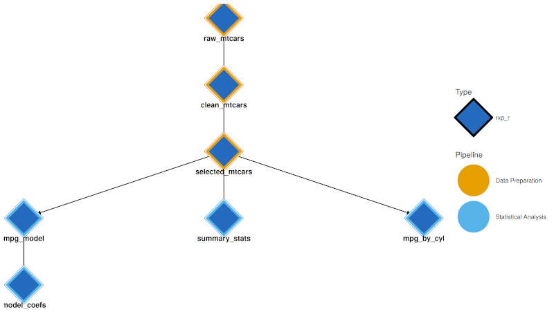
  build = TRUE)

8.2.1 Visualising Sub-Pipelines

When sub-pipelines are defined, visualisation tools use pipeline colours:

1. Interactive Network (rxp_visnetwork()) and Static DAG (rxp_ggdag()) both use a dual-encoding approach:
   • Node fill (interior): Derivation type colour (R = blue, Python = yellow, etc.)
   • Node border (thick stroke): Pipeline group colour This allows you to see both what type of computation each node is and which pipeline it belongs to.

Subpipelines are coloured.

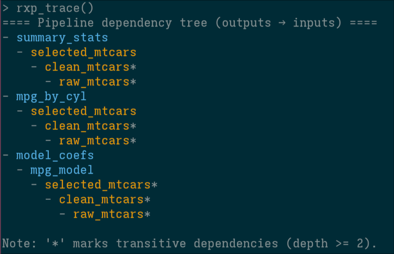
2. Trace: rxp_trace() output in the console is coloured by pipeline (using the cli package).

If your terminal supports it, derivation names are coloured according to the chosen sub-pipeline colour.

It is also possible to not highlight sub-pipelines by using the colour_by argument (allows you to switch between colouring the pipeline, or by derivation type):

rxp_ggdag(colour_by = "pipeline")

rxp_ggdag(colour_by = "type")

8.3 Polyglot Pipelines

One of {rixpress}’s strengths is seamlessly mixing languages. Here’s a pipeline that reads data with Python’s polars, processes it with R’s dplyr, and renders a Quarto report.

TipPolyglot Development Is Now Cheap

Historically, using multiple languages in one project meant significant setup overhead: installing interpreters, managing conflicting dependencies, writing glue code. With Nix, that cost drops to near zero. You declare your R and Python dependencies in one file, and Nix handles the rest.

LLMs lower the barrier further. Even if you are primarily an R programmer, you can ask an LLM to generate the Python code for a specific step, or vice versa. You don’t need to master both languages; you just need to know enough to recognise when each shines. Use R for statistics, Bayesian modelling, and visualisation with {ggplot2}. Use Python for deep learning, web scraping, or leveraging a library that only exists in the Python ecosystem. With Nix handling environments and LLMs helping with syntax, the “cost” of crossing language boundaries becomes negligible.

Open gen-env.R and define the tools your pipeline needs:

library(rix)

rix(
  date = "2026-01-26",
  r_pkgs = c(
    "chronicler",
    "dplyr",
    "igraph",
    "quarto",
    "reticulate",
    "rix",
    "rixpress"
  ),
  py_conf = list(
    py_version = "3.14",
    py_pkgs = c(
      "biocframe",
      "numpy",
      "phart",
      "polars",
      "pyarrow",
      "rds2py",
      "ryxpress"
    )
  ),
  ide = "none",
  project_path = ".",
  overwrite = TRUE
)

The Python packages biocframe, phart, and rds2py are optional but highly recommended when working with ryxpress. biocframe enables direct transfer to polars or Bioconductor DataFrames, bypassing the need for pandas. rds2py (also from the BiocPy project) allows Python to read .rds files, R’s native binary format. Together, these packages ensure seamless interoperability between your R and Python steps. phart is a nice little package that allows you to visualise pipelines from a Python interpreter prompt: not as sexy as R’s {ggdag} but it gets the job done!

8.3.1 Transferring data between Python and R

The rxp_py2r() and rxp_r2py() functions use {reticulate} to convert objects between languages:

rxp_py2r(
  name = mtcars_r,
  expr = mtcars_py
)

However, {reticulate} conversions can sometimes be fragile or behave unexpectedly with complex objects. For robust production pipelines, I recommend using the encoder and decoder arguments to explicitly serialize data to intermediary formats like CSV, JSON, or Apache Arrow (Parquet/Feather).

You can define a custom encoder in Python and a decoder in R:

# Python step: serialize to JSON
rxp_py(
  name = mtcars_json,
  expr = "mtcars_pl.filter(polars.col('am') == 1)",
  user_functions = "functions.py",
  encoder = "serialize_to_json"
),

# R step: deserialize from JSON
rxp_r(
  name = mtcars_head,
  expr = my_head(mtcars_json),
  user_functions = "functions.R",
  decoder = "jsonlite::fromJSON"
)

The Python serialize_to_json function would be defined in functions.py:

#| eval: false
def serialize_to_json(pl_df, path):
    with open(path, 'w') as f:
        f.write(pl_df.write_json())

For larger datasets, Apache Arrow is ideal because it allows zero-copy reads and is supported natively by polars, pandas, and R’s {arrow} package.

Here is how you would transfer data from Python to R:

rxp_py(
  name = processed_data,
  expr = "prepare_features(raw_data)",
  user_functions = "functions.py",
  encoder = "save_arrow"
),

rxp_r(
  name = analysis_results,
  expr = "run_analysis(processed_data)",
  user_functions = "functions.R",
  decoder = "arrow::read_feather"
)

The Python save_arrow encoder function:

#| eval: false
def save_arrow(df: pd.DataFrame, path: str):
    """Encoder function to save a pandas DataFrame to an Arrow file."""
    feather.write_feather(df, path)

Both encoder and decoder functions must accept the object as the first argument and the file path as the second argument. This pattern works for any serialization format supported by your languages of choice.

8.4 Advanced Topics

8.4.1 Complete Polyglot Pipeline Walkthrough

You can find the complete code source to this example over here¹.

For this polyglot pipeline, I use three programming languages: Julia to simulate synthetic data from a macroeconomic model, Python to train a machine learning model and R to visualize the results. Let me make it clear, though, that scientifically speaking, this is nonsensical: this is merely an example to showcase how to setup a complete end-to-end project with {rixpress}.

The model I use is the foundational Real Business Cycle (RBC) model. The theory and log-linearized equations used in the Julia script are taken directly from the excellent lecture slides by Bianca De Paoli.

NoteSource Attribution

The economic theory and equations for the RBC model are based on the following source. This document serves as a guide for our implementation.

Source: De Paoli, B. (2009). Slides 1: The RBC Model, Analytical and Numerical solutions. https://personal.lse.ac.uk/depaoli/RBC_slides1.pdf

First, we need the actual execution environment. Thanks to the {rix} package we can declaratively define a default.nix file. This file locks down the exact versions of R, Julia, Python, and all their respective packages, ensuring the pipeline runs identically today, tomorrow, or on any machine with Nix installed.

#| eval: false
#| code-summary: "Environment Definition with {rix}"
# This script defines the polyglot environment our pipeline will run in.
library(rix)

# Define the complete execution environment
rix(
  # Pin the environment to a specific date to ensure that all package
  # versions are resolved as they were on this day.
  date = "2025-10-14",

  # 1. R Packages
  # We need packages for plotting, data manipulation, and reading arrow files.
  r_pkgs = c(
    "ggplot2",
    "dplyr",
    "arrow",
    "rix",
    "rixpress"
  ),

  # 2. Julia Configuration
  # We specify the Julia version and the list of packages needed
  # for our manual RBC model simulation.
  jl_conf = list(
    jl_version = "lts",
    jl_pkgs = c(
      "Distributions", # For creating random shocks
      "DataFrames", # For structuring the output
      "Arrow", # For saving the data in a cross-language format
      "Random"
    )
  ),

  # 3. Python Configuration
  # We specify the Python version and the packages needed for the
  # machine learning step.
  py_conf = list(
    py_version = "3.13",
    py_pkgs = c(
      "pandas",
      "scikit-learn",
      "xgboost",
      "pyarrow"
    )
  ),

  # We set the IDE to 'none' for a minimal environment. You could change
  # this to "rstudio" if you prefer to work interactively in RStudio.
  ide = "none",

  # Define the project path and allow overwriting the default.nix file.
  project_path = ".",
  overwrite = TRUE
)

Assuming we are working on a system that has Nix installed, we can “drop” into a temporary Nix shell with R and {rix} available:

nix-shell --expr "$(curl -sl https://raw.githubusercontent.com/ropensci/rix/main/inst/extdata/default.nix)"

Once the shell is ready, start R (by simply typing R) and run source("gen-env.R") to generate the adequate default.nix file (or even easier, just Rscript gen-env.R). This is the environment that we can use to work interactively with the code while developing, and in which the pipeline will be executed.

We then need some dedicated scripts with our code. This Julia script contains a pure function that simulates the RBC model and returns a DataFrame. The code is a direct implementation of the state-space solution derived from the equations in the aforementioned lecture and is saved under functions/functions.jl. I don’t show the scripts contents here, as it is quite long, so look for it in the link from before.

At the end of the script, I create a wrapper around Arrow.write() called arrow_write() to serialize the generated data frame into an Arrow file.

While developing, it is possible to start the Julia interpreter and test things and see if they work. Or you could even start by writing the first lines of gen-pipeline.R like so:

library(rixpress)

list(
  # STEP 0: Define RBC Model Parameters as Derivations
  # This makes the parameters an explicit part of the pipeline.
  # Changing a parameter will cause downstream steps to rebuild.
  rxp_jl(alpha, 0.3), # Capital's share of income
  rxp_jl(beta, 1 / 1.01), # Discount factor
  rxp_jl(delta, 0.025), # Depreciation rate
  rxp_jl(rho, 0.95), # Technology shock persistence
  rxp_jl(sigma, 1.0), # Risk aversion (log-utility)
  rxp_jl(sigma_z, 0.01), # Technology shock standard deviation

  # STEP 1: Julia - Simulate a Real Business Cycle (RBC) model.
  # This derivation runs our Julia script to generate the source data.
  rxp_jl(
    name = simulated_rbc_data,
    expr = "simulate_rbc_model(alpha, beta, delta, rho, sigma, sigma_z)",
    user_functions = "functions/functions.jl", # The file containing the function
    encoder = "arrow_write" # The function to use for saving the output
  )
) |>
  rxp_populate(
    project_path = ".",
    build = TRUE,
    verbose = 1
  )

Start an R session, and run source("gen-pipeline.R"). This will cause the model to be simulated. Now, to inspect the data, you can use rxp_read(): by default, rxp_read() will try to find the adequate function to read the data and present it to you. This works for common R and Python objects. But in this case, the generated data is an Arrow data file, so rxp_read(), not knowing how to read it, will simply return the path to the file in the Nix store. We can pass this file to the adequate reader.

rxp_read("simulated_rbc_data") |>
  arrow::read_feather() |>
  head()

Now that we are happy that our Julia code works, we can move on to the Python step, by writing a dedicated Python script, functions/functions.py.

This Python script defines a function to perform our machine learning task. It takes the DataFrame from the Julia step, trains an XGBoost model to predict next-quarter’s output, and returns a new DataFrame containing the predictions. Of course, we could have simply used the RBC model itself for the predictions, but again, this is a toy example.

The Python script contains several little functions to make the code as modular as possible. I don’t show the script here, as it is quite long, but just as for the Julia script, I write a wrapper around feather.write_feather() to serialize the data into an Arrow file and pass it finally to R. Just as before, it is possible to start a Python interpreter as defined in the default.nix file and use to test and debug, or to add derivations to gen-pipeline.R, rebuild the pipeline and check the outputs:

library(rixpress)

list(
  # ... the julia steps from before ...,

  # STEP 2.1: Python - Prepare features (lagging data)
  rxp_py(
    name = processed_data,
    expr = "prepare_features(simulated_rbc_data)",
    user_functions = "functions/functions.py",
    # Decode the Arrow file from Julia into a pandas DataFrame
    decoder = "feather.read_feather"
    # Note: No encoder needed here. {rixpress} will use pickle by default
    # to pass the DataFrame between Python steps.
  ),

  # STEP 2.2: Python - Split data into training and testing sets
  rxp_py(
    name = X_train,
    expr = "get_X_train(processed_data)",
    user_functions = "functions/functions.py"
  ),

  # ... more Python steps as needed ...
) |>
  rxp_populate(
    project_path = ".",
    build = TRUE,
    verbose = 1
  )

Arrow is used to pass data from Julia to Python, but then from Python to Python, pickle is used. Finally, we can continue by passing data further down to R. Once again, I recommend writing a dedicated script with your functions that you need and save it in functions/functions.R. The gen-pipeline.R script would look something like this:

library(rixpress)

list(
  # ... the julia steps from before ...,

  # ... Python steps ...,

  # STEP 2.5: Python - Format final results for R
  rxp_py(
    name = predictions,
    expr = "format_results(y_test, model_predictions)",
    user_functions = "functions/functions.py",
    # We need an encoder here to save the final DataFrame as an Arrow file
    # so the R step can read it.
    encoder = "save_arrow"
  ),

  # STEP 3: R - Visualize the predictions from the Python model.
  # This final derivation depends on the output of the Python step.
  rxp_r(
    name = output_plot,
    expr = plot_predictions(predictions), # The function to call from functions.R
    user_functions = "functions/functions.R",
    # Specify how to load the upstream data (from Python) into R.
    decoder = arrow::read_feather
  ),

  # STEP 4: Quarto - Compile the final report.
  rxp_qmd(
    name = final_report,
    additional_files = "_rixpress",
    qmd_file = "readme.qmd"
  )
) |>
  rxp_populate(
    project_path = ".",
    build = TRUE,
    verbose = 1
  )

To view the plot in an interactive session, you can use rxp_read() again:

rxp_read("output_plot")

To run the pipeline, start the environment by simply typing nix-shell in the terminal, which will use the environment as defined in the default.nix and run source("gen-pipeline.R"). If there are issues, setting the verbose argument of rxp_populate() to 1 is helpful to see the full error logs.

8.4.2 ryxpress: The Python Interface

If you prefer working in Python, ryxpress provides the same functionality. You still define your pipeline in R (since that’s where {rixpress} runs), but you can build and inspect artifacts from Python.

To set up an environment with ryxpress:

rix(
  date = "2025-10-14",
  r_pkgs = c("rixpress"),
  py_conf = list(
    py_version = "3.13",
    py_pkgs = c("ryxpress", "rds2py", "biocframe", "pandas")
  ),
  ide = "none",
  project_path = ".",
  overwrite = TRUE
)

Then from Python:

from ryxpress import rxp_make, rxp_inspect, rxp_load

# Build the pipeline
rxp_make()

# Inspect artifacts
rxp_inspect()

# Load an artifact
rxp_load("mtcars_head")

ryxpress handles the conversion automatically:

• Tries pickle.load first
• Falls back to rds2py for R objects
• Returns file paths for complex outputs

8.4.3 Using rixpress in CI

Running {rixpress} pipelines in Continuous Integration is straightforward. The rxp_ga() function generates a complete GitHub Actions workflow file that handles everything automatically.

To set up CI for your pipeline, simply run:

rxp_ga()

This creates a .github/workflows/ directory with a workflow file that runs your pipeline on every push or pull request.

The generated workflow performs these steps:

1. Restore cached artifacts: If previous run artifacts exist, they are restored using rxp_import_artifacts() to avoid recomputing unchanged derivations.

2. Install Nix: The deterministic Nix installer is used to set up Nix on the runner.

3. Build the environment: Your default.nix environment is built, with the rstats-on-nix cache enabled to speed up R package builds.

4. Generate the pipeline: Your gen-pipeline.R script is executed.

5. Visualise the DAG: Since there’s no graphical interface in CI, the workflow uses stacked-dag (a Haskell tool) to print a textual representation of the pipeline.

6. Build the pipeline: rxp_make() executes, building any derivations that aren’t already cached.

7. Archive artifacts: Build outputs are exported using rxp_export_artifacts() and pushed to a rixpress-runs branch for reuse in subsequent runs.

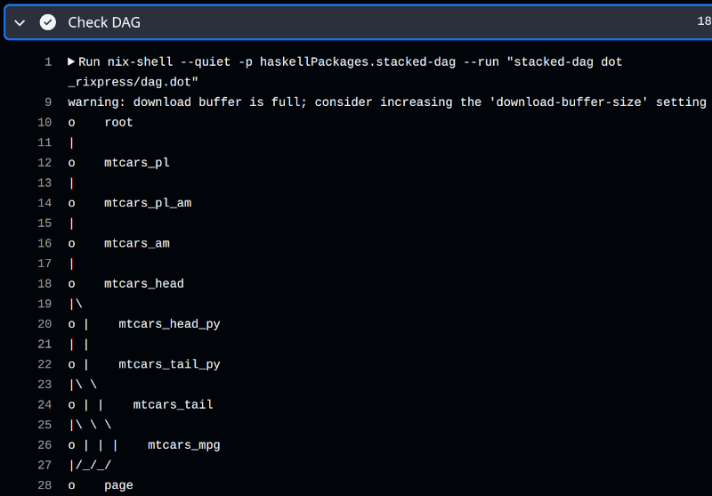
In an interactive session, you would use rxp_ggdag() or rxp_visnetwork() to visualise your pipeline. In CI, the workflow uses stacked-dag to produce a text-based DAG:

- name: Check DAG if dag.dot exists and show it if yes
  run: |
    if [ -f _rixpress/dag.dot ]; then
      nix-shell --quiet -p haskellPackages.stacked-dag \
        --run "stacked-dag dot _rixpress/dag.dot"
    else
      echo "dag.dot not found"
    fi

When rxp_ga() is called, it automatically invokes rxp_dag_for_ci() to generate the required .dot file. The output looks like this:

Text representation of the DAG in CI.

8.4.3.1 Manual Artifact Management

For custom CI setups or sharing artifacts between machines, you can use the export and import functions directly:

# Export all build outputs to a .nar archive
rxp_export_artifacts()

# On another machine or CI run, import before building
rxp_import_artifacts()

By default, artifacts are saved to _rixpress/pipeline_outputs.nar. You can specify a different path:

rxp_export_artifacts(archive_file = "my_outputs.nar")
rxp_import_artifacts(archive_file = "my_outputs.nar")

This approach dramatically speeds up CI by leveraging Nix’s content-addressed storage: if an artifact’s hash matches what’s already in the Nix store, it’s instantly available without rebuilding.

8.4.4 More Examples

The rixpress_demos repository includes:

• jl_example: Using Julia in pipelines
• r_qs: Using {qs} for faster serialization
• python_r_typst: Compiling to Typst documents
• r_multi_envs: Different Nix environments for different derivations
• yanai_lercher_2020: Reproducing a published paper’s analysis

8.5 Caveats: Consequences of Hermetic Builds

Nix derivations are hermetic: they run in an isolated sandbox with no network access and a minimal, reproducible filesystem. This design ensures reproducibility but has practical implications:

No network access during builds. If your analysis requires downloading data from an API or remote source, this must happen before the pipeline runs. Use rxp_r_file() or rxp_py_file() to read pre-downloaded data, or create a separate script outside the pipeline to fetch data into a data/ directory.

Environment variables must be explicit. Tools that rely on environment variables (like CmdStan for Bayesian modelling) need these set via the env_var argument. For example, CmdStanR requires pointing to the CmdStan installation:

rxp_r(
  name = model_fit,
  expr = fit_stan_model(data),
  user_functions = "functions.R",
  env_var = c(CMDSTAN = "${defaultPkgs.cmdstan}/opt/cmdstan")
)

See vignette("cmdstanr", package = "rixpress") for a complete Bayesian workflow example.

Paths are relative to the build sandbox. Files referenced in your code must be explicitly included via additional_files or user_functions. The build environment doesn’t see your working directory—only what you declare.

8.6 Summary

{rixpress} unifies environment management and workflow orchestration:

• Define pipelines with rxp_*() functions in familiar R syntax
• Mix languages freely: R, Python, Julia, Quarto
• Build with Nix for deterministic, cached execution
• Inspect outputs with rxp_read(), rxp_load(), rxp_copy()
• Debug with timestamped build logs
• Share reproducible pipelines via Git

The Python port ryxpress provides the same experience for Python-first workflows.

By embracing structured, plain-text pipelines over notebooks for production work, your analysis becomes more reliable, more scalable, and fundamentally more reproducible.

---

1. https://github.com/b-rodrigues/rixpress_demos/tree/master/rbc